Facilitate advanced waveguide layout definitions and optimization tasks via a powerful Python interface
Model straight and bent waveguides and fibers made of dispersive, anisotropic, and lossy materials
Model multi-mode, multi-core, and photonic crystal optical fibers
Model uni- and bidirectional electromagnetic field propagation and scattering matrices for 2D and 3D photonic devices
Verify cross-sections and device layouts and analyze results using advanced and highly customizable visualization capabilities
Integrate with the circuit-level simulator VPIcomponentMaker Photonic Circuits
Powerful Object-Oriented Python Interface
Python provides easy to learn and feature-rich object-oriented programming environment
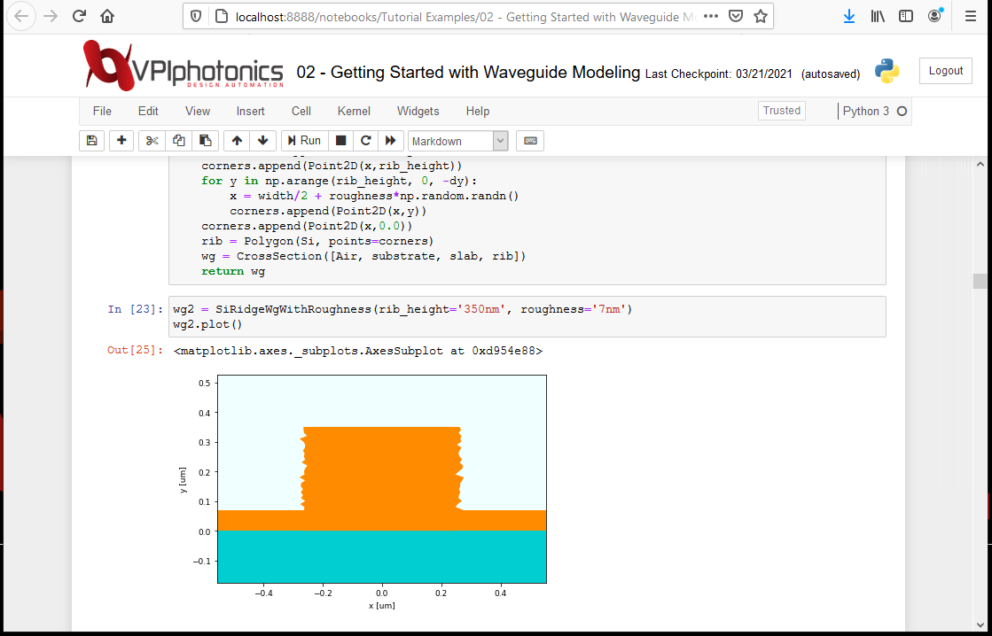
User-friendly Jupyter Notebook and Juypter Lab environments allow combining interactive simulation scripts with results, figures, problem descriptions, and equations
Integration with the SciPy – ecosystem of Python open-source libraries enables advanced
visualization and mathematical, scientific, and engineering computations
Finite-Difference Optical Mode Solvers
Full-vectorial and semi-vectorial finite-difference 2D mode solvers for straight and bent anisotropic and isotropic channel waveguides and fibers
Specialized finite-difference 1D mode solver for straight and bent planar waveguides
Support of nondiagonal anisotropy for straight waveguides
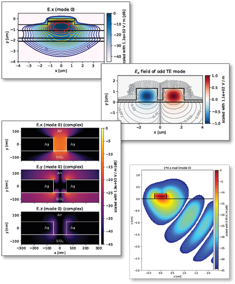
Handling of electric field singularities near sharp corners of plasmonic and high-index contrast waveguides
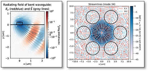
Calculation of guided and leaky modes (leakage to substrate, leakage due to bending)
Support of perfectly matched layer (PML) boundaries
Symmetric perfect electric or magnetic conductor (PEC, PMC) boundary conditions
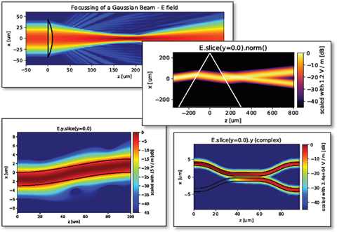
BPM and EME Solvers for Modeling Photonic Devices
Calculation of electromagnetic field propagation in 2D and 3D photonic devices
Extraction of scattering matrices for multi-port photonic devices
Support of arbitrary excitation sources:
• Port modes and their superpositions
• Gaussian beams and plane waves
• User-defined fields
Beam Propagation Method (BPM)
Full-vectorial and semi-vectorial finite-difference 2D and 3D BPM schemes
Uni-directional field propagation
Paraxial and wide-angle approximations
Absorbing PMLs and transparent boundary conditions
Efficient for devices with low refractive index contrast and smoothly varying cross-sections
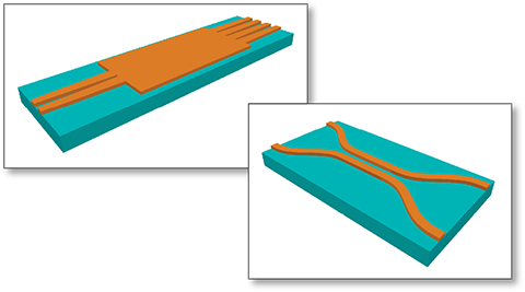
Application examples: tapers, S-bends, directional couplers, ring couplers, Y-splitters
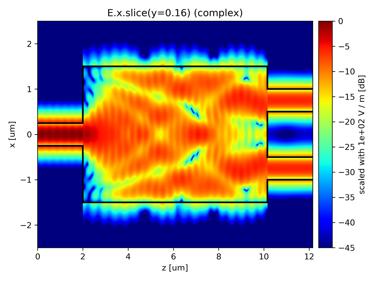
Eigenmode Expansion (EME) Method
Based on full-vectorial finite-difference mode solvers
Bi-directional field propagation handling back reflections
Efficient for device length optimization, devices with high refractive index contrast and step-like varying cross-sections
Application examples: multi-mode interference (MMI) couplers and reflectors, waveguide-based polarization and mode converters
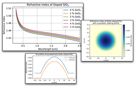
Advanced Fiber Material Models
Built-in dispersive doped silica material model with an extendible library of dopants (predefined are GeO₂, B₂O₃, F, Cl).
Support of uniform and non-uniform dispersive materials to define step-index and graded-index fibers
Obtain doping concentration profiles from imported measured refractive index profiles
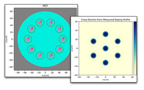
Flexible and Multicore Fiber Layouts
Define arbitrary fiber cross-section geometries (circular, elliptic, hexagonal, or other shapes)
Create fiber cross-sections from measured refractive index or doping profiles
Dedicated support of multicore fiber layouts: cores can be individually activated and deactivated to investigate individual core modes, supermodes, and inter-core coupling
Fiber Mode Calculation and Analysis
Scalar and vectorial 2D finite-difference mode solvers
Native support of bent fiber modes and bent mode losses
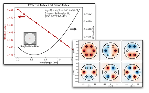
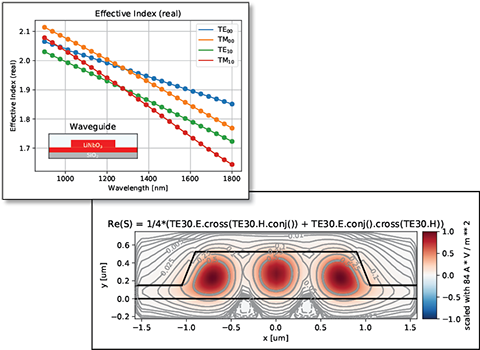
Analyze and visualize the effective index and the modal fields Ψ or E and H
Predict datasheet parameters using IEC- and ITU-compliant parameter definitions:
• group index, dispersion, dispersion slope
• zero dispersion wavelength, zero dispersion slope
• cutoff wavelength (theoretical, fiber, cable)
• mode field diameter (near field and far field)
• numerical aperture, effective mode area
Calculate inter-core mode coupling coefficients in multicore fibers with arbitrary cross-sections
Dispersive, Lossy and Anisotropic Optical Materials
Single-line definition of dispersionless lossy optical materials
Native support of Sellmeier, Lorentz-Drude, Tauc-Lorentz, and Cody-Lorentz models of dispersive materials
Easy definition of arbitrary measured and analytical frequency dependences for refractive index or dielectric permittivity, absorption, and thermo-optic coefficient
Easy definition of dispersive anisotropic optical materials (including gyrotropic birefringence and magneto-optic effect)
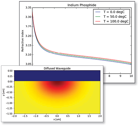
Easy definition of dispersive graded-index optical materials for modeling graded-index fibers and diffused waveguides
Library of predefined dispersive and thermo-optic materials (Air, Silicon, Silica, Si3N4, InP, LiNbO3, and standard metals)
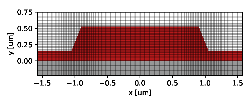
Customizable Nonuniform Finite-Difference Meshing
Built-in adaptive quasi-uniform mesh
Uniform, quasi-uniform, and stretched meshes in user-defined layout areas
Arbitrary user-defined nonuniform meshes
Sub-pixel averaging of discretized dielectric constant
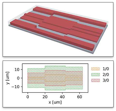
Flexible Layout Generation
GDS mask import and export:
• Extrude complete 3D layered components from imported GDS masks
• Extract 2D fabrication masks from designed and optimized 3D layouts
• Support of fabrication-aware corrections for sidewall angles, expansion or shrinkage, and inversion
• Powerful filtering and transformation of points, enabling geometry sweeps on GDS-imported layouts
Creation of 3D waveguides, tapers, S-bends, etc. from 2D waveguide cross-sections
Built-in 2D and 3D geometry library for primitive shapes, geometrical transformations, and Boolean operations
Creation of arbitrarily complex 3D shapes by loading them from STL files
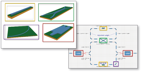
Advanced visualization of 2D and 3D shapes, layouts, and layout cross-sections
Parametric Modeling with Automated Sweeps
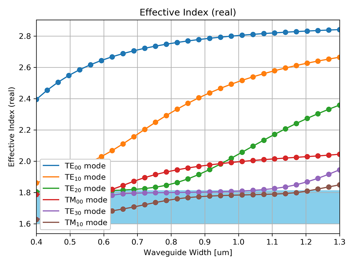
Easy sweeping of wavelength and one more arbitrary model parameter (e.g., waveguide width, bend radius, mesh resolution, or refractive index)
Flexible interface for calculating additional user-defined mode properties during sweeps
Automated fitting or interpolation of sweep results
Plotting a mode property vs. the sweep parameter is easy—correct axis labels and legend entries are created automatically
Mode Properties Analysis
Immediate access to dispersive waveguide properties (group mode index, group velocity dispersion, and dispersion slope) as well as mode attenuation, effective mode area, custom user-defined properties, and vectorial mode fields
Easy calculation of mode expansion coefficients, mode overlap integrals, optical coupling efficiency, mode power, and other characteristics
Electric and magnetic fields are Python objects natively supporting mathematical operations such as field superposition and scaling, scalar and vector products, etc.
Advanced Plotting Capabilities
Built-in field interpolation and visualization
Single-line plot methods for a quick overview of results
Highly configurable field plots supporting field lines, contour lines, density plots, etc.
Access to underlying Matplotlib objects for additional plot customization
Interoperability and Data Export
Export guided mode properties and device scattering matrices for use in VPIcomponentMaker Photonic Circuits
Save your results (guided modes and fields) to reuse them later without recalculation
Utilize Python's power and flexibility to postprocess and export results for the desired target application